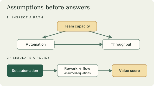
1 · Inspect causal paths
Explore the original project map, or load “Common cause: team capacity”. There, capacity affects both automation and throughput. Compare the open path with and without conditioning on capacity.
Green dashed arrow: directed route · Rust arrow: displayed back-door route · Gold box: collider on a displayed path · double border: conditioned · dashed box: unobserved
Trace the paths
“Open” means d-connected on this path under the selected conditioning set. A back-door path begins with an arrow into X; some are already blocked. An open path does not prove a nonzero effect.
Overview: from boxes to assumptions
A directed acyclic graph (DAG) represents a proposed causal story. An arrow asserts a direct influence relative to the variables included. The original map keeps Scope Creep, Interface Misalignment, Vendor Capacity, Design Risk, Delay and Cost Overrun. Edit it to expose disagreements before analysing it.
Quick background: chains, forks and colliders
A chain X → M → Y carries a directed causal route. A fork X ← C → Y can create association through a common cause. In X → C ← Y, C is a collider on that path. Conditioning on C, or a descendant of C, opens that route unless another non-collider blocks it. A variable can be a collider on one path and a non-collider on another.
A directed path is not the “front-door criterion”. This tool does not implement front-door identification.
What is the adjustment test?
For Pearl’s back-door criterion, the set contains no descendants of X and blocks all paths beginning with an arrow into X. This lesson tests that criterion exactly and lists all inclusion-minimal observed sets: removing any member would invalidate the set. “Minimal” need not mean the fewest variables.
The calculation removes outgoing arrows from X and checks d-separation. It assumes the graph is correct, including its missing arrows, and uses explicit unobserved nodes rather than bidirected edges. It does not test data quality, overlap/positivity, consistency or the truth of those assumptions. If no observed set passes this sufficient criterion, the effect may still be identifiable by another method.
2 · Simulate programme policies
A fictional delivery team has 52 weeks of staffing, automation, WIP limits and outcomes. Fit the stated equations, then compare a fixed baseline with changed controls. This is an intervention simulation under assumptions, not a recovered counterfactual for a real week.
The assumed flow
S · A · W
Throughput T
Defects D
2T − 0.03L − 1.5D
Unplanned work U is external to the policy. R depends on U,A,W,S; T on S,A,U,R,W; L on W/T; D on U,R,A,T. The value score is a chosen trade-off, not money or a validated programme objective.
Baseline
Outcome distributions
Green = selected policy; gold outline = baseline. Histograms show simulation counts; the score plot shows 5th–95th percentiles and an interquartile box. These spreads omit coefficient and model uncertainty; they are not confidence intervals.
Policy comparison
Each option uses the same random draws. A zero change therefore has exactly zero simulated difference. All controls are fixed at baseline means plus the requested changes; “baseline” is itself a model scenario, not the observed history.
Data preview and fitted equations
Overview / one minute
Choose a policy and inspect its simulated throughput, lead time and defects. Compare the presets, then try a custom change. These results can help frame questions for a small, measured trial. They cannot select a proven best policy for a real programme.
Imported telemetry changes the fitted coefficients. It does not validate the causal story or make the proposed action equivalent to a randomised experiment.
Manager and analyst view
The model fixes staffing S (FTE), automation A (0–1) and WIP cap W (items). It draws an unplanned-work index U, then rework index R, throughput T (items/week), lead time L (days) and defects D (defects/item). It scores each draw using the original weights 2, −0.03 and −1.5.
Costs of extra staffing or automation are absent. Rank changes are conditional on those chosen weights and the model. Examine the outcome columns, observed input ranges, clipping counts and sensitivity to assumptions before proposing a trial. Smaller spread alone does not establish a safer intervention.
Full model and uncertainty assumptions
R := c0 + c1·U + c2·A + c3·W + c4·S + εR
T := a0 + a1·S + a2·A + a3·U + a4·R + a5·W + εT
L := b0 + b1·W/T + εL
D := d0 + d1·U + d2·R + d3·A + d4·T + εD
Separate least-squares regressions fit the four equations. Simulation assumes invariant equations and independent Gaussian errors with fitted residual standard deviations. U uses the sample mean and sample standard deviation, with negative draws set to zero. Policies share the same shocks for a reproducible comparison. Error independence, linearity, stable units and the absence of omitted confounding are assumptions, not regression findings. Time dependence and changing regimes are omitted.
Controls are bounded at S ≥ 0, A ∈ [0,1], W ≥ 1. Simulated values are floored at R,D ≥ 0, T ≥ 0.05 items/week and L ≥ 0.1 days. These are declared numerical modelling choices; extensive clipping is a warning about model mismatch. Least squares fits the unclipped equations, so clipping changes their simulated means. Zero-noise propagation is not the mean of a nonlinear simulation.
The lead-time equation is an empirical WIP-cap proxy. Little’s law concerns average occupancy = flow rate × average time under appropriate stable-system conditions. A WIP limit is not measured occupancy, and W/T in weeks requires a time conversion to days. The fitted intercept and slope absorb a local empirical relation; no queueing identity is enforced here.
A unit counterfactual needs evidence-conditioned abduction of the unit’s disturbances, an action, then prediction with those disturbances. This app samples new scenarios and performs no such abduction. Coefficient uncertainty, causal identification, formal influence-diagram optimisation, EVPI/VOPI, budget constraints and SLA optimisation remain outside this trial.
Run small model checks
These browser checks are smoke checks. The repository also tests graph criteria against an independent path oracle and regressions against known solutions.